Reinforcement Learning
Supervised and unsupervised learning are the two most widely studied and researched branches of Machine Learning (ML). Besides these two, there is also a third subcategory in ML called Reinforcement Learning (RL). The three branches have fundamental differences. Supervised learning for example is designed to learn from a training set of labeled data, where each element of the training set describes a certain situation and is linked to a label/action the supervisor has provided [Ham18]. On the other hand, RL is a method in which the machine tries to map situations to actions by maximizing a reward signal [ADBB17]. The two methods are fundamentally different from each other in the fact that in RL there is no supervisor which provides the label/action the machine needs to take, rather there is a reward system set up from which the machine can learn the correct action/label [Ham18]. Contrarily to supervised learning, unsupervised learning tries to find hidden structures within an unlabeled dataset. This might seem similar to RL as both methods work with unlabeled datasets, but RL tries to maximize a reward signal instead of finding only hidden structures in the data [ADBB17]. Unsupervised learning on the other hand learns about how the data is distributed [SBLL19].
RL finds its roots in multiple research fields. Each of these fields contributes to the RL in its own unique way [Ham18]. For example, RL is similar to natural learning processes where the learning method is by experiencing many failures and successes. Therefore psychologists have used RL to mimic psychological processes when an organism makes choices based on experienced rewards/punishments [EWC21]. While psychologists are mimicking psychological processes, neuroscientists are using RL to focus on a well-defined network of regions of the brain that implement value learning [EWC21]. In Robotics it is used to help learn drones fly in mid-air [AKAM+21]. RL finds also applications in health care, Natural Language Processing, Management of Limited Resources, etc… [NRC20]. The main subfields of RL are presented in Figure 1. The reason why RL can be applied to a range of research fields is that it uses a natural learning process based on a trial and error method as we will see in the next subsection.
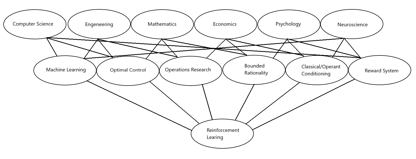
Fig. 1 research fields involved in reinforcement learning
Finite Markov Decision Processes
RL can be represented in finite Markov Decision Processes (MDPs), which are classical formalizations of sequential decision making. More specifically, MPDs give rise to a structure in which delayed rewards can be balanced with immediate rewards [SB18]. Moreover, it enables a straightforward framing for learning from an environment to achieve a goal [Lev18]. In its simplest form, RL works with an Agent-Environment Interface. The agent is exposed to some representation of the environment’s state \(S_t \in \mathrm{S}\). From this representation the agent needs to choose an action \( A_t \in \mathcal{A}(s)\), which will result in a numerical reward \(R_{t+1} \in \mathbb{R} \) and a new state \(S_{t+1}\) (see Figure 2) [SB18]. The goal for the agent is to learn a mapping from states to action called a policy \(\pi\) that maximizes the expected rewards:
If the MPDs are finite and discrete, the sets of states, actions, and rewards (\(S\), \(A\), and \(R\)) all have a finite number of elements. The agent-environment interaction can then be subdivided into episode [ADBB17]. The agent’s goal is to find the policy which maximizes the expected discounted cumulative return in the episode [FranccoisLHI+18].
Where T indicates the terminal state and \(\gamma\) is the discount rate. The terminal state \(S_T\) is often followed by a reset to a starting state or sample from a starting distribution of states [FranccoisLHI+18]. An episode ends once the reset has occurred. The discount rate represents the present value of future rewards. If the dicount rate is zero \(\gamma = 0\), the agent is myopic and is only concerned with maximizing the immediate rewards. The agent can consequently be considered greedy [SBLL19]. If the returns are rewritten in a dynamic programming approach, the return of the myopic agent becomes:
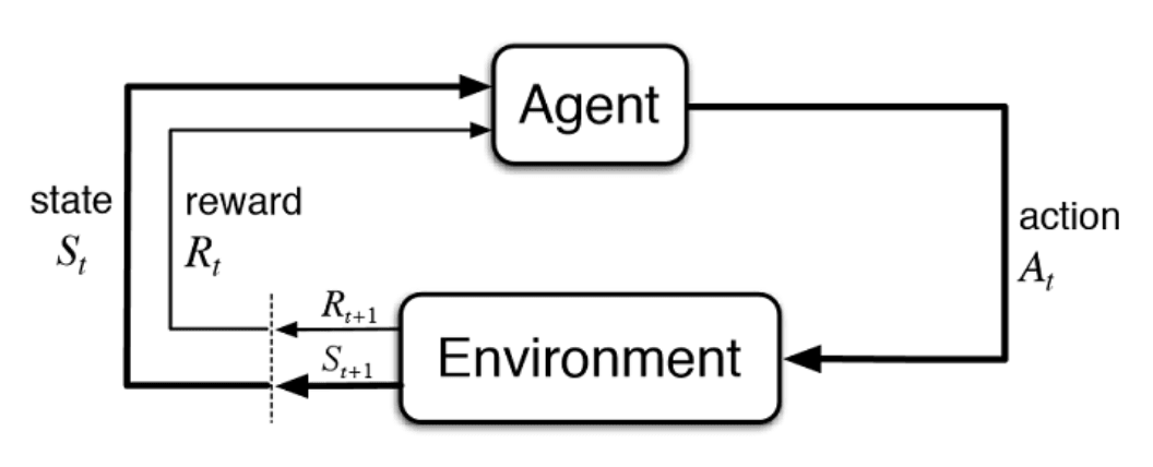
Fig. 2 standard model reinforcement learning
A key concept of MPDs is the Markov property: Only the current state affects the next state [FranccoisLHI+18]. The random variables \(R_t\) and \(S_t\) have with the Markov property well defined discrete transition probability distributions dependent only on the previous state and action:
For all \(s', s \in \mathrm{S} , r \in \mathbb{R}, a \in \mathrm{A}(s) \). The probability of each element in the sets \(S\) and \(R\) completely characterizes the environment [SB18]. This is an unrealistic assumption to make, and several algorithms relax the Markov property. The Partial Observable Markov Decision Process (POMDP) algorithm, for example, maintains a belief over the current state given the previous belief state, the action taken, and the current observation [ADBB17]. Once \(p\) is known, the environment is fully described and functions like a transition function \(T : D \times A \to p(S)\) and a reward function \(R: S \times A \times S \to \mathbb{R}\) can be deducted [SB18].
Most algorithms in RL use a value function to estimate the value of a given state for the agent. Value functions are defined by the policy \(\pi\) the agent decided to take. As mentioned previously, \(\pi\) is the mapping of states to actions. More precisely, the policy \(\pi\) provides us with the probability of selecting the action \(a\) given the state \(s\). The value function also describes the probability of a reward given the action taken and by consequence, the value function \(v_{\pi}(s)\) in a state \(s\) following a policy \(\pi\) is as follows:
This can also be rewritten in a dynamic programming approach:
Equation (4) is called the Bellman equation of \(v_{\pi}\). It describes the relationship between the value of a state and the values of its successor states given a certain policy \(\pi\). The relation can also be represented by a backup diagram (see Figure 3). If \(v_{\pi}(s)\) is the value of a given state, then \(q_{\pi}(s,a)\) is the value of a given action of that state:
This can be seen in the backup diagram as starting from the black dot and computing the subsequent value thereafter. \(q_{\pi}(s,a)\) is also called the action-value function as it describes each value of an action for each state.
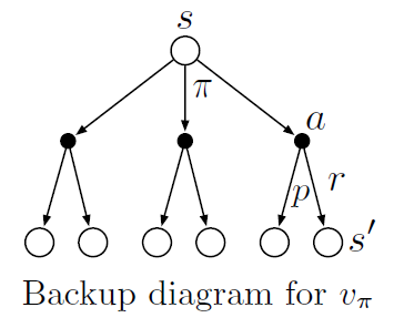
Fig. 3 General backup diagram
For the agent, it is important to find the optimal policy which maximizes the expected cumulative rewards. The optimal policy \(\pi_*\) is the policy for which \(v_{\pi_*}(s) > v_{\pi}(s)\) for all \(s \in S\). An optimal policy also has the same action-value function \(q_*(s,a)\) for all \(s \in S\) and \(a \in A\). The optimal policy does not depend solely on one policy and can encompass multiple policies. It is thus not policy dependent:
Once \(v_*(s)\) is found, you need to apply a greedy algorithm as the optimal value function already takes into account the long-term consequences of choosing that action. Finding \(q_*(s, a)\), makes things even easier, as the action-value function caches the result of all one-step-ahead searches.
Solving the Bellman equation such that we know all possibilities with their probabilities and rewards is in most practical cases impossible. Typically this is due to three main factors [SB18]. The first problem is obtaining full knowledge of the dynamics of the environment. The second factor is the computational resources to complete the calculation. The last factor is that the states need to have the Markov property. To circumvent these obstacles, RL tries to approximate the Bellman optimality equation using various methods. In the next chapter, a brief layout of these methods is discussed, focussing on the methods applicable for financial planning.
Generalized Policy Iteration, Model-based RL and Model-free RL
A general theory in finding the optimal policy \(\pi_*\) is called Generalized Policy Iteration (GLI). This method is applied to almost all RL algorithms. The main idea behind GLI is that there is a process that evaluates the value function of the current policy \(\pi\) called policy evaluation and a process that improves the current value function called policy improvement [SB18], [VOW12]. To find the optimal policy these two processes work in tandem with each other as seen in Figure 4 [VOW12]. Counterintuitively, these processes also work in a conflicting manner as policy improvement makes the policy incorrect and it is thus no longer the same policy [SB18], [BHB+20]. While policy evaluations create a consistent policy and thus the policy no longer improves upon itself. This idea runs in parallel with the balance between exploration and exploitation in RL. If the focus lies more on exploration, the agent frequently tries to find states which improve the value function. However, putting more emphasis on exploration is a costly setting as the agent will more frequently choose suboptimal policies to explore the state space. If exploitation is prioritized, the agent will take a long time to find the optimal policy as the agent is likely not to explore new states to improve the policy [VOW12]. An \(\varepsilon\)-greedy algorithm is a good example of an algorithm where the balance between exploration and exploitation is important (see next subsection).
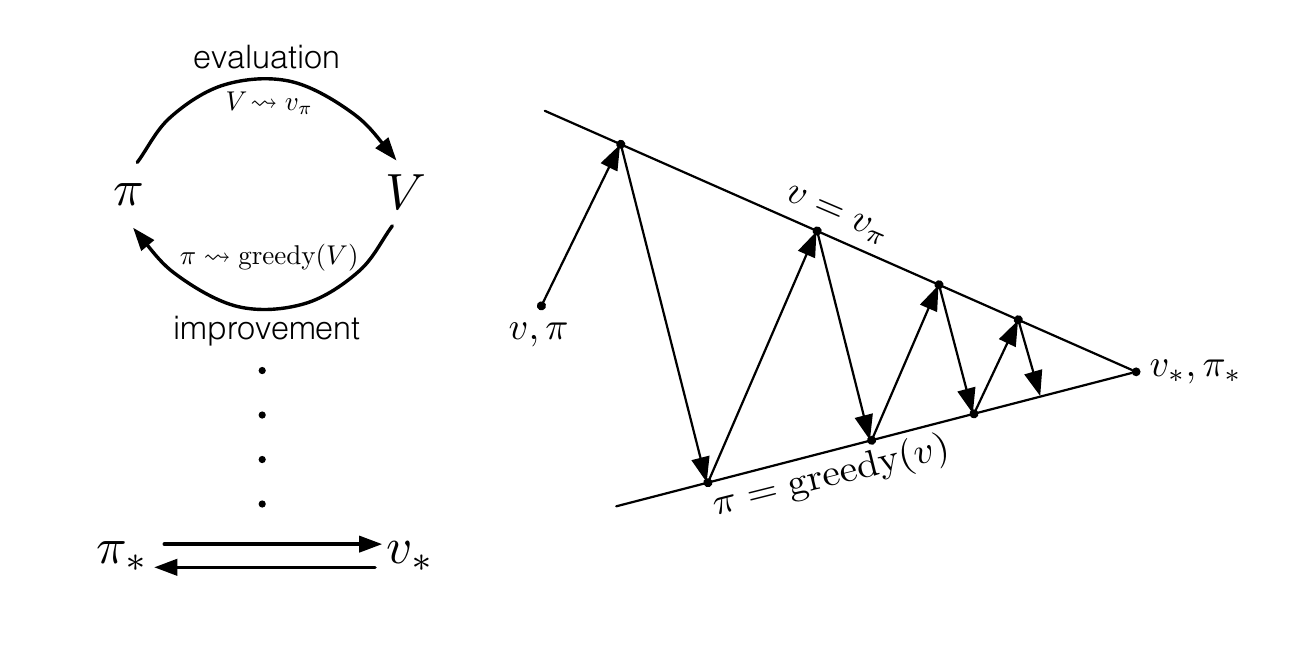
Fig. 4 Generalized policy iteration
Reinforcement Learning can be subdivided between model-based RL and model-free RL. In model-free RL the dynamics of the environment are not known. \(\pi_*\) is found by purely interacting with the environment. Meaning that these algorithms do not use transition probability distribution and reward function related to MDP [FranccoisLHI+18]. Moreover, model-free RL has irreversible access to the environment. Meaning the algorithm has to move forward after an action is taken [MBJ20b]. Model-based RL on the other hand has reversible access to the environment because they can revert the model and make another trail from the same state [MBJ20a]. Good examples of model-free RL techniques are the Q-learning and Sarsa. They tend to be used on a variety of tasks, like playing video games and learning complicated locomotion skills [SB18]. Model-free RL lay at the foundation of RL and the first algorithms to be applied in RL were model-free RL techniques. On the other hand, model-based RL is developed independently and in parallel with planning methods like optimal control and the search community as they both solve the same problem but differ in the approach [WZZ19]. Most algorithms in model-based RL have a model which describes the dynamics of the environment. They improve the learned value or policy function by sampling from the model [MBJ20a] (see Figure 5). This enables the agent to think in advance and as it were plan for possible actions. Model-based reinforcement learning finds thus large similarities with the Planning literature and as a result, a lot of cross-breeding between the two is happening. For example, an extension of the POMP algorithm called Partially Observable Multi-Heuristic Dynamic Programming (POMHDP) is based on recent progress from the search community [KSL19]. A hybrid version of the two approaches in which the model is learned through interaction with the environment, has also been widely applied. The imagination-augmented agents (12A) for example combine model-based and model-free aspects by employing the predictions as an additional context in a deep policy network [MBJ20b]. In the next subsection, three fundamental algorithms in RL are discussed which will enable us to better capture the dimensions and challenges of RL algorithms.
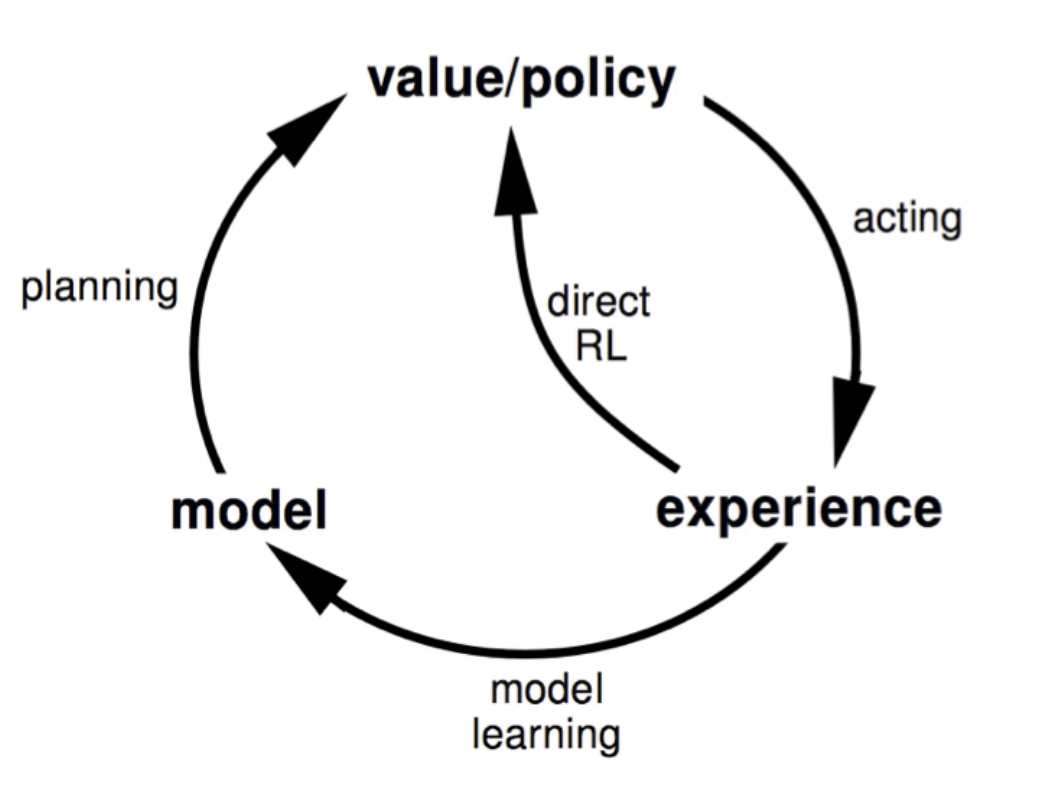
Fig. 5 Model-based Reinforcement Learning
Dynamic Programming, Monte Carlo Methods and Temporal-Difference Learning
The three most fundamental algorithms for RL are Dynamic Programming, Monte Carlo method ,and Temporal-difference Learning. Dynamic Programming (DP) is known for two algorithms in RL: value iteration (VI) and policy iteration (PI). For both methods, the dynamics of the environment need to be completely known and therefore, they fall under model-based RL. The two algorithms also use a discrete-time, state ,and action MDP as they are iterative procedures. The PI can be subdivided into three steps: initialize, policy evaluation ,and policy improvement [VOW12]. The first step is to initialize the value function \(v_{\pi}\) by choosing an arbitrary policy \(\pi\). The following step is to evaluate the function successively by updating the Bellman equation (4). Updating the Bellman equation is also called the expected update as the equation is updated using the whole state space instead of a sample of the state space. One update is also called a sweep, as the update sweeps through the state space. Once that the value function \(v_{\pi}\) is updated, we know how good it is to follow the current policy. The next step is to deviate from the policy trajectory and choose a different action \(a\) in state \(s\) to find a more optimal policy value. We compute the new \(\pi '\) and compare it to the old policy. The new policy is accepted if \(\pi '(s) > \pi(s)\). This process is repeated until a convergence criterion is met [PRD96]. The complete algorithm can be found in the appendix. VI combines the policy evaluation with the policy improvement by truncating the sweep with one update of each state. It effectively combines the policy evaluation and policy evaluation in one sweep (see appendix for the algorithm) [PRD96] . PI and VI are the foundation of DP and numerous adaptions have been made to these algorithms. Although these algorithms do not have a wide application in many fields, they are essential in describing what an RL algorithm effectively tries to approximate [SB18].
The Monte Carlo (MC) methods do not assume full knowledge of the dynamics of the environment and are thus considered model-free RL techniques. They only require a sample sequence of states, actions ,and rewards from the interaction of an environment. Technically, a model is still required which generates sample transitions, but the complete probability distribution \(p\) of the dynamic system is not necessary. The idea behind almost all MC methods is that the agent learns the optimal policy by averaging the sample returns of a policy \(\pi\) [ADBB17]. They can therefore not learn on an online basis as after each episode they need to average their returns. Another difference between the two methods is that the MC method does not bootstrap like DP [MJ20]. Meaning, each state has an independent estimate. Note that Monte Carlo methods create a non-stationary problem as each action taken at a state depends on the previous states. MC methods can either estimate \(a\) state value (3) or estimate the value of a state-action pairs (5) (recall that the state-action values are the value of an action given a state). If state values are estimated, a model is required as it needs to be able to look one step ahead and choose the action which leads to the best reward and next state. With action value estimation you already estimated the value of the action and no model needs to be taken into account. Monte Carlo methods also use a term called visits. A visit is when a state or state-action pair is in the sample path. Multiple visits to a state are possible in an episode. Two general Monte Carlo Methods can be deducted from visits. The every-visit MC methods and the first-visit MC methods. The every-visit MC methods estimate the value of a state as the average of the returns that have followed all visits to it. The first visit method only looks at the first visit of that state to estimate the average returns [VOW12]. The biggest hurdle in MC methods is that most state-action pairs might never be visited in the sample.
To overcome this problem multiple solutions were explored. The naïve solution to this problem is called the exploring starts. Here, the idea is to allocate to each action in each state a nonzero probability at the start of the process. Although this is not possible in a practical setting where we truly want to interact with an environment, it enables us to improve the policy by making it greedy with respect to the current value function. As each state has a certain probability to explore, it will eventually explore the complete state space. If then an infinite number of episodes are taken, the policy improvement theory states that the policy \(\pi\) will convergence to the optimal policy \(\pi_*\) given the exploring starts [Dol10]. Two other possibilities are applied in the field to solve this problem: on-policy methods and off-policy methods [SB18]. On-policy methods attempt to improve on the current policy. This is also called a soft policy as \(\pi(a|s) > 0\) for all \(s \in S\) and all \( a \in A(s)\), but shifts eventually to the deterministic optimal policy. One of these on-policy methods is called an \(\varepsilon\)-greedy policy. The \(\varepsilon\)-greedy policy uses with probability \(\varepsilon\) a random action instead of the greedy action. \(\varepsilon\) is a fine-tuning parameter as it sets the balance between exploration and exploitation. The \(\varepsilon\)-soft policy is thus also a compromised solution as one cannot exploit and explore at the same rate. This is re-elected by the fact that the \(\varepsilon\)-greedy policy is the best policy only among the \(\varepsilon\)-soft policies. The pseudocode of on-policy first visit MC for \(\varepsilon\)-soft policies algorithm can be found in the appendix. Lastly, the off-policy methods can be applied to overcome both the unrealistic exploring starts and the compromise needed in the on-policy methods. Off policy methods solve the exploration versus exploitation dilemma by considering two separate policies [VOW12]. one policy, called the target policy \(\pi\), is being learned to become the optimal policy ,and another policy, called the behavior policy \(b\), generates the behavior to explore the state space. In an off-policy method there needs to be coveraged between the behavior policy and the target policy to transfer the exploration done by behavior policy \(b\) to the target policy \(\pi\). Meaning, every action taken under \(\pi\) also needs to be taken occasionally under \(b\). Consequently, the behavior policy needs to be stochastic in states where it deviates from the target policy. Complete coverage would imply that the behavior policy and the target policy are the same. The off-policy method would then become an on-policy method. The on-policy method can thus be viewed as a special case of off-policy in which the two policies are the same. Most off-policy methods use importance sampling to estimate expected values under one distribution given samples from another. Importance sampling uses the ratio of returns according to the relative probability of the trajectories of the target and behavior policies to learn the optimal policy [MVHS14]:
The formula is called the importance-sampling ratio. Note that the ratio only depends on the two policies and the sequence, not on the MDP. The importance-sampling ratio effectively transforms the expectations of \(v_b(s)\) to have the right expectation. Now, we can effectively estimate \(v_{\pi}(s)\):
Where \(J(s)\) are all time steps in which state \(s\) is visited for an every-visit MC method and for a first-visit MC method \(J(s)\) are all time steps that were first visits to state \(s\). An alternative to importance sampling is weighted importance sampling in which a weighted average is used:
The advantage of using a weighted importance sampling is a reduced variance as the variance is bounded when a weighting scheme is applied. The downside of this technique is that it increases the bias as the expectation deviates from the expectation of the target policy [MVHS14].
The last general method to talk about is Temporal-difference Learning (TD). Temporal-difference Learning is a hybrid between Monte Carlo methods and Dynamic Programming. As DP, it updates estimates based on other learned estimates, not waiting on the final outcome, but it can learn directly from experience without a model of the environment like MC methods [SB18]. The simplest TD method is the one-step TD. It updates the prediction of \(v_{\pi}\) at each time step:
While MC method would update after each episode:
One-step TD effectively bootstraps the update like DP, but it uses a sampling estimate like the MC method to estimate V [RMM18]. The sampling estimate differs from the expected estimate on the fact that they are based on a single sample successor rather than on the complete distribution of all possible successors [KC21]. In the updating rule of TD methods there is the TD error (see quantity in brackets) which is the difference between the previous estimate of \(S_t\) and the updated estimate \(R_{t+1} + \gamma V(S_{t+1})\). The TD error is the error in the estimate made at that time. The pseudocode of the one-step TD method can be found in the appendix. TD methods lend themselves quite easily to different methods in MC. For example, the Sarsa control algorithm is an on-policy TD in which the action values are updates using state-action pairs [KC21]:
The same methodology is used here. \(q_\pi\) is continuously estimated for policy \(\pi\) while policy \(\pi\) changes toward the optimal policy \(\pi^*\) by a greedy approach. TD methods can also be applied to off-policy fashion. They are then called Q-learning which is widely applied in the literature. Q-learning is an off-policy method because they learn the action-value function \(q\) independent of the policy being followed. They select the maximal or minimal action-value pair in the current state \(s\):
The policy still has an effect in that it determines which states-action pairs are being visited, but the learned action-value function \(q\) directly approximates \(q_*\). This simplifies the analysis and enables early convergence. The last TD method is called the expected Sarsa and it uses the expected value instead of the minimum over the next state-action pairs to update the value function:
The main benefit of Expected Sarsa over Sarsa is that it eliminates the variance caused by the random selection of \(a_{t+1}\). Another benefit of Expected Sarsa is that it can be used as an off-policy method when the target policy \(\pi\) is replaced with another policy [San21].
These three methods lay at the foundation of RL and numerous adaptations have been made to fit the problem at hand. For example, Adaptive Dynamic Programming is implemented to approximate the original dynamic programming equations [WZL09]. In Figure 6 the backup diagrams of the three different methods are represented. From the backup diagrams, it becomes clear that each algorithm approaches GPI from a different perspective. In the following subsection the different elements in a RL algorithm are explored.
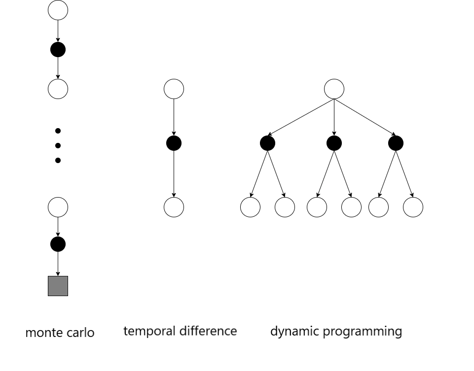
Fig. 6 The backup diagrams of Monte Carlo, Temporal-difference Learning and Dynammic Programming
Dimensions of a Reinforcement Learning Algorithm
Moerland et al. [MBJ20a] addresses the six most critical dimensions of an RL algorithm: computational effort, action value selection, cumulative return estimation, policy evaluation, function representation ,and update method. These dimensions give a clear overview of the ability of RL algorithms to adapt to different situations. The first dimension has to do with the computational effort that is required to run the algorithm. The computational effort is primarily determined by the state set that is chosen (see Figure 7). The first option is to consider all states \(S\) of the dynamic environment. In practice, this often becomes impractical to consider due to the curse of dimensionality. The second and third possibilities are all reachable states and all relevant states. All reachable states are the states which are reachable from any start under any policy, while for the relevant states only those states under the optimal policy are considered. The last option is to use start states. These are all the states with a non-zero probability under \(p(s_0)\). The curse of dimensionality is further discussed in the next subsection as it is one of the primary challenges in RL.
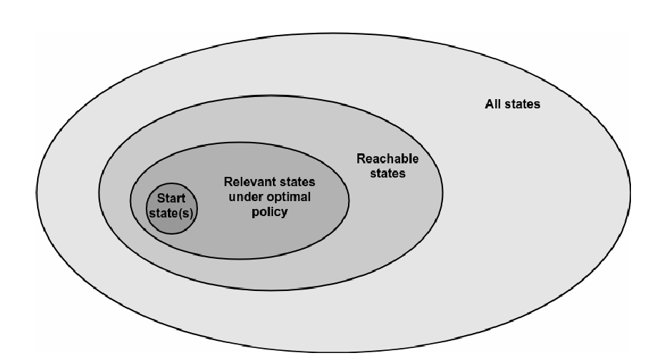
Fig. 7 state_space dimensions
The second dimension is the action selection and has primarily to do with exploration process of the algorithm. The first consideration in action selection is the candidate set that is considered for the next action. Then the optimal action needs to be considered while still keeping exploration in mind. For selecting the candidate set two main approaches are considered: step-wise and frontier. Frontier methods only start exploration once they are on the frontier of the iteration, while step-wise methods have a new candidate set at each step of the trajectory. The MC method, DP ,and TD learning described above use step-wise exploration, while frontier methods are primarily used in robotics [NZKN19]. For the second consideration, selecting the action value, different methods have been adopted. The first one is random explorations like \(\varepsilon\)-greedy exploration as explained in the section of Monte Carlo methods. These explorations techniques enable us to escape from a local minimum but can cause a jittering effect in which we undo an exploration step at random. The second approach is a value-based exploration that uses the value-based information to better direct the perturbation [YLL+19]. A good example of this are mean action values. They improve the random exploration by incorporating the mean estimates of all the available actions. Meaning, they explore actions with higher values more frequently than actions with lower values. The last option is state-based exploration. State-based exploration uses state-dependent properties to inject noise. Dynamic programming is a good example of this approach. DP is an ordered state-based exploration. Ordered state-based exploration sweeps through the state space in an orded like tree structure. Other state-based explorations are possible like novelty and priors.
The dimensions of the calculation of the cumulative return estimation (see (1)) can be expressed in an other formula to address the practical issues and limitations in RL:
where \(T \in {1,2,3, ..., \infty}\) denotes the sample depth and \(B(.)\) is a bootstrap function. For the sample depth three possible option are possible: \(K = \infty\), \(K = 1\), \(K = n\) or reweighted. Monte Carlo methods for example use a sample depth to infinity as they do not bootstrap at all. Instead, DP uses bootstrapping at each iteration, so \(K = 1\). An intermediate method between DP and Monte Carlo methods can also be devised in which \( K = n\). The reweighted option is a special case of \( K = n\) in which targets of different depths are combined with a weighting scheme. The bootstrap function can be devised using a learned value function like the state value function or the state-action value function or following a heuristic approach. A good heuristic can be obtained by first solving a simplified version of the problem. An example of this is first solving the deterministic problem and then using the solution as a heuristic on its stochastic counterpart [MBJ20a]. The second dimension in cumulative return estimation is whether full knowledge of the dynamic system is in place (full backups) or a sample is taken from the environment (sample backups) [ADBB17]. In Figure 8 these two dimensions are represented.
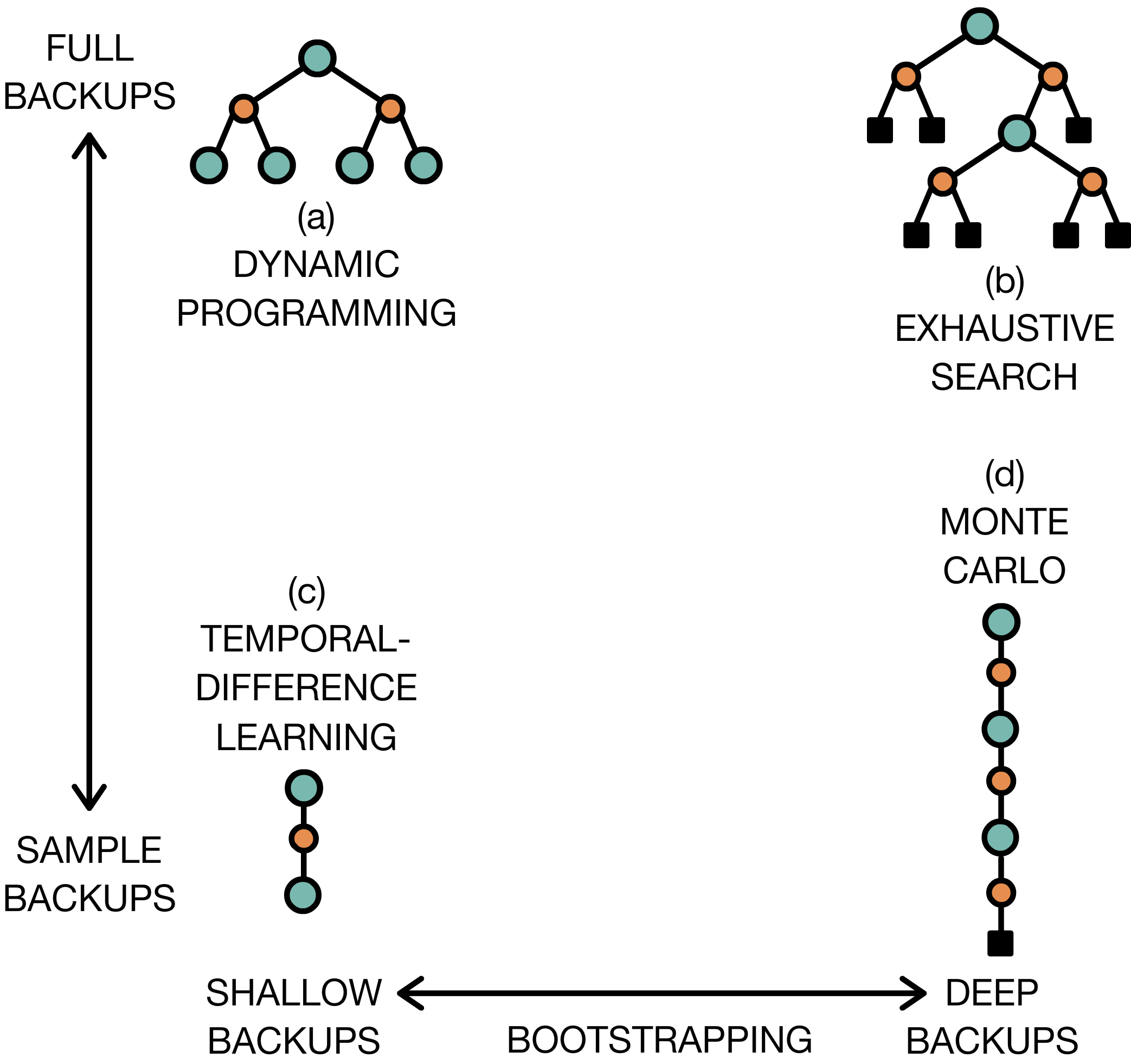
Fig. 8 consideration in calculating the cumulative return estimation
The fourth dimension to consider is policy evaluation. Policy evaluation has to do with which policy to use: on-policy or off-policy method. We have already seen this dimension in the section of MC methods and it will not be further discussed. Another dimension is function representation. The first choice that needs to be made here is which function to represent. In theory, we have two essential functions: the value function and the policy function. The value function can be the state-action value function or just the state value function, but primarily represents the value of the current or optimal policy at all considered state-action pairs. The policy function on the other hand maps every state to a probability distribution over actions and is best used in continuous action spaces as we can directly act in the environment by sampling from the policy distribution [MBJ20a]. The second choice is how to represent this function. There are two possibilities here. The first option is using a tabular approach in which each state is a unique element for which we store an individual estimate. This can be done on a global level or local level. At the global level, the entire state space is encapsulated by the table. Unfortunately, this method does not scale well and is only relevant in small exploratory problems. On the contrary, a local table does scale well as it is built temporarily until the next real step. The other method for function representation is function approximation. Function approximation builds on the concept of generalization. Generalization assumes that similar states to function will in general also have approximately similar output predictions (Generalization is further discussed in the next section). Function approximation uses this to share information between near similar states and therefore store a global solution for a larger state space [VOW12]. There are two kinds of function approximations: parametric and non-parametric. A good example of a parametric function approximation is a neural network and for non-parametric a k-nearest neighbors can be thought of. The big challenge in function approximation is finding the balance between overfitting and underfitting the actual data.
The last dimension is the updating method. The updating method used should be in line with the function representation and the policy evaluation method as certain updating rules only work on a set of function representation and policy evaluation methods [MBJ20a]. For the updating method, there are quite a few choices to make. The first choice is choosing between gradient-based updates and gradient-free updates. In gradient-based updates we repeatedly update our parameters in the direction of the negative gradient loss with respect to the parameters:
where \(\alpha \in \mathbb{R}^+\) is a learning rate. Before the updating rule can be applied a loss function \(L(\theta)\) should first be chosen. The loss function is usually a function of both the function representation and the policy evaluation method. As there are two kinds of function to represent in function representation, there are also two kinds of losses: value loss and policy loss. The most general value loss is the mean squared error loss. In policy loss, there are various methods to estimate the loss. For example the policy gradient specifies a relation between the value estimates \(\hat{q}(s_t,a_t)\) and the policy \(\pi_{\theta}(a_t|s_t)\) by ensuring that actions with high values also get high policy probabilities assigned:
Once the loss function is defined, the gradient-based updating rule can be applied. The updating again depends on the function representation for example the value update on a table for the mean squared loss function becomes:
where \(q(s,a)\) is a table entry. The same can be done for function approximation where the derivative of the loss function then becomes:
where \(\frac{\partial q(s,a)}{\partial \theta}\) can be for example the derivatives in a neural network.
Gradient-free updating rules use a parametrized policy function and then repeatedly perturb the parameters in policy space, evaluate the new solution by sampling traces and decide whether the perturbed solution should be retained. they only require an evaluation function and treat the problem as a black-box optimization setting. Gradient-free updating methods are thus not fit for model-based RL. An overview of the different dimensions can be viewed in Figure 9.
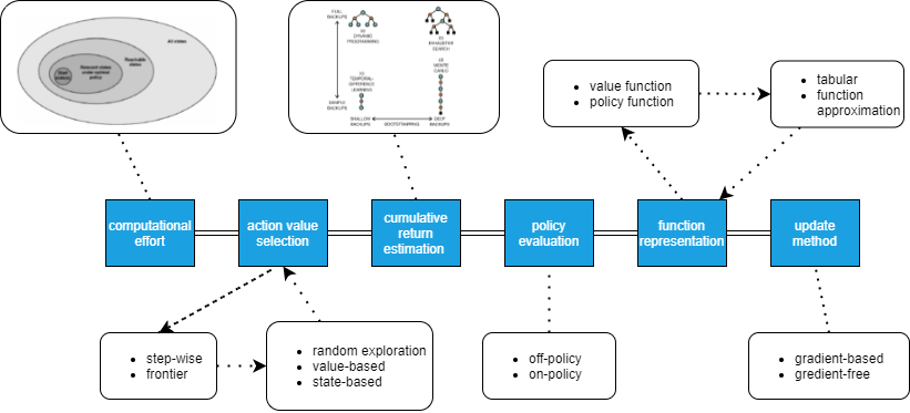
Fig. 9 The dimensions of a reinforcment learning algorithm
Curse of Dimensionality and generalization
If the state space is small, a tabular approach can be used to represent each state or state-action pair in a separate cell. This is very tractable because the states can be stored in a table. Unfortunately, this method becomes infeasible once the state space increases in size as the number of states grows exponentially larger with the number of state variables. Also, when the action and state space are continuous, we have an infinite amount of possible state-action pairs to explore, making the tabular approach impossible [SBLL19]. This is called the curse of dimensionality. To tackle the issue, RL borrows a technique from supervised learning called generalization. In RL generalization refers either to
the capacity to achieve good performance in an environment where limited data has been gathered
the capacity to obtain good performance in a related environment
In the first case, the agent needs to behave optimally in a similar environment as the trained one. Here, the notion of sample efficiency is important. In the latter case, there are patterns between the trained and test environments and the agent needs to transfer its learning from one environment to the other. This is also called transfer learning and meta-learning [FranccoisLHI+18].
To better grasp the concept of generalization, consider an i.i.d. sampled dataset \(D\) as a set of four-tuples \(\{s,a,r,s'\} \in S \times A \times R \times S \) available to the agent. Where \(D_{\infty}\) is the data set where the number of tuples tends to infinity. Then a learning algorithm is a mapping of a dataset \(D\) into a policy \(\pi_D\), where the suboptimality of the policy’s expected return can be decomposed as follows:
The decomposition consists of the asymptotic bias and the overfitting term. The asymptotic bias is independent of the quantity of the data and is caused by how the \(\pi_{D_{\infty}}\) is computed. In contrast, the overfitting term is directly related to the size of the dataset and measures the error caused by a limited amount of data. The goal of the policy \(\pi_D\) is to minimize the suboptimality as efficiently as possible. Improving the suboptimality is challenging due to the trade-off between the asymptotic bias and the overfitting term. For example, if there is a significantly large state space, we cannot visit every state-action pair and therefore have a limited amount of data. Meaning, the error in our estimate is primarily caused by the overfitted term. The overfitting term can be reduced by introducing asymptotic bias. This will in turn significantly reduce the error caused by the small dataset, but also introduce a biased estimator [FranccoisLHI+18]. The most used technique in the literature to introduce bias is function approximations. These techniques will be discussed in the next subsection together with the challenges of using function approximations.
Function Approximation
Function approximations attempt to generalize by taking examples from the desired function and then constructing an approximation of the function using those examples. So instead of using a table in which the states are stored, a parametrized functional form with weight vector \(w \in R^d\) is used to represent the function. So for example, the value and state-value function can be approximated by
\(v\) can be approximated by \(\hat{v}\) using for instance a linear function in features of state \(s\) given a weight vector \(w\) of the features weight. Another possibility is using a decision tree, where \(w\) is all the numbers defining the split points and leaf values of the tree. The most notable function approximations are neural networks. Especially deep neural networks (DNN) can significantly reduce the time and effort required to approximate the value function [SBLL19]. The approximation functions used in supervised learning are not always suitable in an RL environment. The reason for this is that supervised learning methods like decision trees and multivariate regression are used in a static environment where the model is only learning from a prespecified dataset. Contrarily to supervised learning, RL methods learn while interacting with an environment and thus need to learn efficiently from incremental data [San21]. In addition, RL requires function approximation methods to be able to handle non-stationary target functions, because we often seek to learn \(q_{\pi}\) while \(\pi\) is changing. Even if the policy remains the same, the target values of training examples are non-stationary if they are generated by bootstrap methods (DP, TD learning) [SB18].
As discussed in the previous section, function representation such as function approximation and table approach have a large impact on the updating rule applied. If a look-up table is used, the update is trivial as the table entry for \(s\)’s estimated value has simply been shifted a fraction to the update target \(u\). All the values of the other states are in this case left unchanged. However, with function approximation we generalize the states by representing many states with weights (see Figure 10). Meaning, an update at one state affects many others, and it is thus not possible to get the values of all states correct. The problem of having more states than weights is resolved by a state distribution \(\mu (s) \geq 0, \sum_s \mu(s) = 1\). The state distribution specifies which states are important by applying a weight to the error of the state [San21]. Once a weight is giving to each state’s error, a mean squared value error is applied which tells us how good the function approximation is representing the value function:
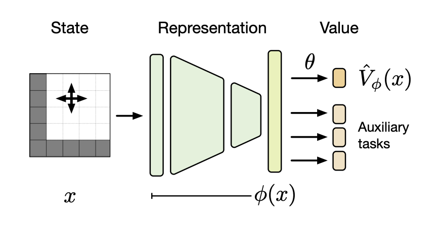
Fig. 10 general approach of function approximation methods
Now we have discussed the general working of function approximation, a closer look is given to linear gradient-descent methods and artificial neural networks (ANN). Linear gradient descent methods and ANN are two popular function approximations used in RL. Although there are many other techniques like Coarse Coding and memory-based function approximation, it is impossible to cover all function approximations. We will therefore only look at linear-gradient descent methods. One of the linear gradient descent methods is the stochastic-gradient descent (SGD). In SGD the weight vector is a column vector with fixed number of real-valued components \(w = (w_1, w_2,..., w_d)^{\top}\) and the approximate value function \(\hat{v}(s,w)\) is a differentiable function of w for all \( s \in S\). The weight vector is updated at each time step \(t=0,1,2,3,...\), giving us \(w_t\). By interacting with the environment, we get a new example \(S_t \rightarrow v_{\pi}(S_t)\) giving us a state \(S_t\) and the value under the policy. The goal of the function approximation is to approximate the value of the state with limited resources. Meaning from the example, we generalize to all other states while upholding an accurate representation of the seen state. SGD methods do exactly that they minimize the error observed on the examples by adjusting the weight vector after each example by a small amount in the direction that would reduce the error in that example the most:
where \(\alpha\) is a positive step-size parameter, and \(\Delta \hat{v}(S_t, w_t)\) is the column vector of partial derivatives of the expression with respect to the components of the vector. This can be written for any scale expression \(f(w)\) that is a function of a vector \(w\):
The gradient of \(f\) with respect to \(w\) determines the optimal directions in which the error falls most rapidly and \(\alpha\) determines the step size in the direction of the gradient. The step size is an important parameter to set as it sets up the balance between accuracy on the example and the generalization property. More specifically, we do not want the error of the example to be zero as that would decrease the quality of the generalization to other states. Instead, the step size should incorporate the generalization by decreasing \(\alpha\) to zero over time. Then, by combining small updates over many examples, the SGD method creates the ability to minimize an average performance measure such as the \(\overline{VE}\). Following this property, the SGD method is guaranteed to converge to a local optimum. The SGD method is called stochastic because we implement the update on a single example [BI99].
In most cases, the true value, \(v_{\pi}(S_t)\), is not the target output. Rather, some approximation to it like a noise corrupted version of \(v_{\pi}(S_t)\) or a bootstrapping target using \(\hat{v}\). If the target value is not the exact update because \(v_{\pi}(S_t)\) is unknown, we can approximate it by substituting \(U_t\) in place of \(v_{\pi}S_t\). \(U_t\) needs to be an unbiased estimate , \(\mathbb{E}[U_t|S_t=s] = v_{\pi}(s)\). Unfortunately, the bootstrapping method of estimating \(v_{\pi}(S_t)\) is biased because it is estimated on the current value of the weight vector \(w_t\). As a result, they only include a part of the gradient. Namely, they take into account the effect of changing the weight vector \(w_t\) on the estimate but ignore its effect on the target. Therefore, they are called semi-gradient methods. In the next paragraph, the SGD update is combined with a linear approximate function [GP13].
The linear method approximates the state-value function by the inner product between \(w\) and \(x(s)\)
where the vector \(x(s)\) is called a feature vector representing state \(s\) and \(w\) is the weight vector. For linear function approximations, it is natural to use the SGD updates. The gradient then becomes
and the SGD update reduces to
By specifying the feature vector, it is possible to add domain knowledge to a reinforcement learning system. The features should therefore correspond to the aspects of the state space.
A limitation of the linear function approximation is that it cannot incorperate interaction between features. A possible solution to the problem are polynomial features as higher-order polynomial bases allow for more accurate approximations of more complicated functions. Also, nonlinear function approximations like an artificial neural network can be used.
Most of the function approximations that are discussed above relate to on-policy RL. For off-policy RL function, approximation methods are more challenging as the distribution of the update becomes a difficult concept in which two policies need to factor in the generalization aspect. The main intuition behind the problem is that the behavior policy might select actions which the target policy would never select. This can cause divergence because no update is made on these actions (the importance sampling ratio is zero). Consequently, the off-policy method expects higher rewards but does not actually know whether there are higher rewards after the action as there was no update to check this creating divergence. A lot of research is still needed in this area to solve the divergence problems of off-policy methods. For instance, the Baird’s counterexample is one of the big hurdles of finding a general concept of convergence for off-policy learning methods. Also, the combination of function approximation, bootstrapping ,and off-policy training is called the deadly triad as combining these three elements can give rise to the danger of instability and divergence. Unfortunately, all these three elements give rise to significant advantages ,and giving up on one of these elements is sometimes not preferred [SB18].
Function approximation is a subfield in RL which is one of the main drivers behind the recent advances in the field. With state-of-the-art function approximation techniques, more complex environments can be tackled. This can give rise to more advanced applications of RL in domains like optimal control, robotics ,and financial planning. In the next subsection, an adaptation of Q-learning is discussed, called G-learning.
G-learning, a stochastic adaptation on Q-learning
Q-learning learns extremely slow in noisy environments due to the minimization bias. In (7) the minimum over the estimated values is used implicitly as an estimate of the minimum value, which can lead to a significant positive bias in noisy environments. Consider, for example, a single state \(s\) where there are many actions \(a\) whose true values are all zero but whose estimated values are uncertain and thus distributed some above and some below zero. The minimum of the true values is zero, but the minimum of the estimates is negative. Consequently, introducing minimization bias {cite}´sutton2018reinforcement´. This can also be illustrated by the Jensen’s inequality for the concave min operator. Assume that \(Q(s,a)\) is an unbiased but noisy estimate of the optimal \(Q^*(s,a)\). Then it applies that
This creates an optimistic bias, causing the cost-to-go to appear lower than it is. The minimization bias has an impact on the learning rate of the Q-learning policy. The impact depends on the gap \(Q^*(s,a') - V^*(s)\) between the value of a non-optimal action \(a'\) and that of the optimal action. If the gap is large, \(a'\) seems suboptimal as desired. If the gap is small, confusing \(a'\) for the optimal action does not affect the learning process. However, when the gap is in the order of the noise term, the minimization bias has a significant impact, because \(a'\) does not appear to be suboptimal and is thus still accepted as optimal. The optimistic bias is further enhanced by propagating the bias between states and can lead to regions of the state space that are highly biased creating large-gap suboptimal actions. Although this problem hampers the learning rate, Q-learning can still learn in a stochastic environment since the bias draws exploration towards the given state, leading to a decrease in variance, which in turn reduces the bias [FPT15].
G-learning is an adaptation of Q-learning constructed by Fox et all [FPT15]. It is designed to handle noisy environments. It is also an off-policy approach in a model-free setting, but it regularizes the state-action value function learned by an agent. It regularizes the state-action value function by penalizing deterministic policies early in the optimization process. Penalization is done early in the process because there is still a small sample size and therefore a more randomized policy is preferred. When the sample size grows, one should expect to shifts to a more deterministic and exploiting policy. This is what G-learning effectively does. It adds a cost-to-go term to the value function that penalizes the early deterministic policies which diverge from a simple stochastic prior policy \(\pi_0(a|s)\). The prior stochastic policy sets up an information cost of a learned policy \(\pi(a|s)\), effectively penalizing deviations from the prior policy. G-learning is therefore called an entropy regularization of Q-learning.
Taken the expectation of the policy \(\pi\) gives us the Kullback-Leibler divergence of the two policies.
Now consider the total discounted expected information cost
Adding (11) to the value function (3) gives the free-energey function
where \(\beta\) is the parameter that sets the weight of the information cost in the value function. If \(\beta\) is small, \(\pi\) will act similar to \(\pi_0\). When \(\beta\) is large, \(\pi\) will diverge from the prior and will therefore approach the greedy policy of Q-learning. A smooth transition between small and large values for \beta will allow the algorithm to avoid early deterministic policies and still be able to exploit the optimal values. The same approach can be done for the state-action value function \(q(s,a)\)
Notice that the information term at time \(t=0\) is not needed as the action \(a_0 =a\) is already known. Given (12) and (13), it follows that
The gradient of \(F^{\pi}\) at zero is
Equation (15) is the soft-min operator applied to H. Now evaluate (14) at (15)
This expression can get plugged in (13) and as a result the optimal \(H^*\) is achieved.
The G-learner is used in the first application for a retirement plan optimization problem. In the next subsection, we will describe the general approach of the Deep BSDE method and link it to the RL theory. The Deep BSD method is applied to solve high-dimensional terminal Partial Differential Equation (PDE), which a lot of optimal control problems in finance struggle to solve.
The Deep Backward Stochastic Differential Equation Method
There are many financial control problems that need to solve a partial differential equation to obtain the optimal solution and some financial planning applications are no different. The Deep BSDE method is an RL inspired approach to solve terminal PDEs in higher dimensions. The general PDEs that the Deep BSDE method solves can be written as:
with some terminal condition \(u(T,x) = g(x)\).
The key idea is to reformulate the PDE as an appropriate stochastic problem [HJ+20] and [WHJ17]. Here, the probability space (\(\Omega,\mathcal{F}, \mathbb{P}\)) is adapted to the high dimensional problem. So, \(W: [0, T] \times \Omega \rightarrow \mathbb{R}^d\) becomes a d-dimensional standard Brownian motion on (\(\Omega,\mathcal{F}, \mathbb{P}\)) and let \(\mathcal{A}\) be the set of all \(\mathcal{F}\)-adapted \(\mathcal{R^d}\)-values stochastic processes with continuous sample paths. Let \(\{X_T\}_{0 \leq t \leq T}\) be a d-dimensional stochastic process which satisfies
Using Itô’s lemma, we obtain that
A forward-backward stochastic differential equation can be written as
In the literature it was found that the solution of PDE and its spatial derivative are now the solution of the stochastic control problem (19) [HJ+20]. The relationship between the PDE (18) and the BSDe (19) is based on the nonlinear Feynman-Kac formula [Blo18] and [GulerLP19]. Under suitable additional regularity assumption on the nonlinearity \(f\) in the sense that for all \(t \in[0,T]\) it holds \(\mathbb{P}\)-a.s. that
The first identity in (20) is referred to as nonlinear Feynman-Kac formula [WHJ17]. The pair \((Y_t, Z_t), t \in [0,T]\) is a solution for the BSDE and with (20) in mind, the PDE problem can be formulated as the following variational problem:
The minimizer of this variational problem is the solution to the PDE [Rai18]. The main idea behind Deep BSDE method is to approximate the unknown function \(X_0 \rightarrow u(, X_0)\) and \(X_t \rightarrow [\sigma(t,X_t)]^T((\Delta_x u)(t,X_t)\) by two feedforward neural networks \(\psi\) and \(\phi\) [HJW18]. To achieve this, we discretize time using Euler scheme on a grid \( 0 = t_0<t_1<...<T_N =T \)
At each time slide \(t_n\), a subnetwork is associated. These subnetworks are then stacked together to form a deep composite neural network [HJW17]. The network takes the paths \(\{X_{t_n}\}_{0\leq n \leq N}\) and \(\{W_{t_n}\}_{0\leq n \leq N}\) as the input data and gives as final output, denoted by \(\hat{u}(\{ X_{t_n}\}_{0 \leq n \leq N}, \{W_{t_n}\}_{0 \leq n \leq N})\), as an approximation to \(u(t_N, X_{t_N})\) (see Figure 11) [HJW18]. Thereby it is only solved a time step \(t=0\). The difference in the matching of a given terminal condition can be used to define the expected loss function [HJ+20] [HJW17].
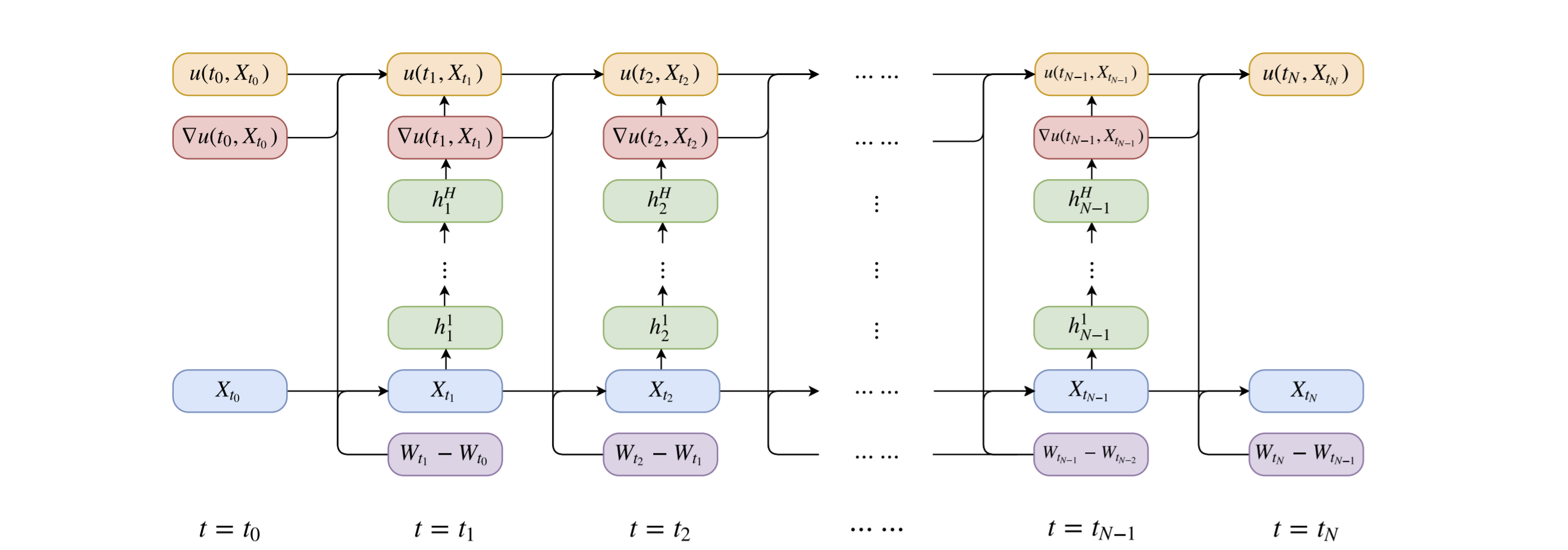
Fig. 11 neural network for Deep BSDE method
Another way to look at it is that the stochastic control problem is a model-based reinforcement learning problem [HJW18]. In this setting, the gradient \(Z\) is viewed as the policy we try to approximate using a feedforward neural network. The process \(u(t, \varepsilon + W_t), t \in [0, T]\), corresponds to the value function associated with the stochastic control problem and can be approximately employed by the policy Z [WHJ17]. A benefit of using the Deep BSDE method is it does not require us to generate training data beforehand. The paths play the role of the data and they are generated on the spot [HJ+20].
The Deep BSDE method solves the PDE for \(Y_0= u(0, X_0) = u(0, \varepsilon)\). This means that in order to obtain an approximate of \(Y_t = u(t,X_t)\) at a later time \(t>0\), we will have to retain our algorithm. Although this method is originally designed to only solve the equation at time step \(t=0\), future research might be able to solve the PDE at each time point \(t\).